
Chapter 7: Equilibrium and Newton’s First Law

Equations introduced and used for this topic (all equations can be written and solved as both scalar and vector and all equations are generally solved as vectors):
∑ Fx, y, z = 0 NT = r x F
T clockwise = T counter-clockwise
(m1 + m2) xcm = m1x1 + m2x2
Where
T is the Torque, measured in Newton-Metres (Nm)
F is Force, measured in Newtons (N)
r is the length of the lever-arm measured in Metres (m)
m1 & m2 are the masses of two bodies, measured in kilograms (kg)
xcm , x1 and x2 are the distances, measured in metres (m)
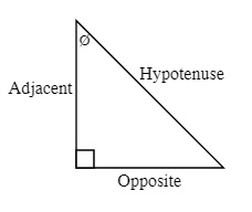
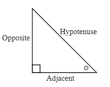
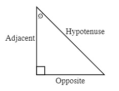
ø is the angle given for the triangle and is generally between the Adjacent Side and the Hypotenuse with the angle measured in degrees (be careful to make sure that the calculator is not working in gradients or radians).
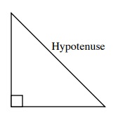
Hypotenuse is the longest side in a right triangle and is opposite to the 90° angle
Opposite is the side that is opposite to the angle that you are given
Adjacent is the side that is beside the angle you are given
The Trigonometric Functions
[latex]Sine Ø =\dfrac{Opposite}{Hypotenuse}[/latex] [latex]Cosine Ø =\dfrac{Adjacent}{Hypotenuse}[/latex] [latex]Tangent Ø =\dfrac{Opposite}{Adjacent}[/latex]
7.1 Right Angle Trigonometric Functions 4, 5

Trigonometry, a term derived from the Greek trigonon (triangle) and metron (measure) has historical roots dating back 4000 years to writings found in Egyptian and Babylonian mathematics and astronomical records. Indian astronomers were using trigonometry over 2600 years ago and widespread usage by Islamic and Chinese mathematicians was common at least 1500 years before that.
The study of trigonometry returned to European nations in the Renaissance from translations of Arabic and Greek writings. Modern trigonometry reached its current form through the works of Leonard Euler (1707-1783), who is considered one of the greatest mathematicians in history and worked in nearly every area of mathematics and physics. Modern notation used in trigonometry comes directly from Euler’s writings, as do many other currently used notations in mathematics and physics. Euler’s achievements and writings that have been collected in 92 volumes, making him one of the most prolific writers in mathematics history.
- Not sure about his #4 footnote. Is it for the triangles? I went to the Hulton archive and did not find any pictures for these triangles. Same for Google.
Introductory trigonometry is based on the similarities between identical right angled triangles (one angle is 90°) of different sizes. If the angles of triangles are identical then all of these triangles are simply larger or smaller copies of each other.
If you take any two sides of any triangle shown above and divide them by each other, that number will be exactly the same for the same two sides chosen from any of the triangles.
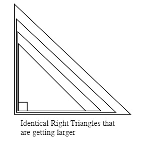
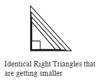
In all of the cases shown above if you take any two sides of any triangle shown and divide them by each other, that number will be exactly the same for the same two sides chosen from any of the triangles.
These triangle ratios have defined names:
[latex]Sine =\dfrac{Opposite}{Hypotenuse}[/latex] [latex]Cosine =\dfrac{Adjacent}{Hypotenuse}[/latex] [latex]Tangent =\dfrac{Opposite}{Adjacent}[/latex]
You often see these equations shortened to:
[latex]Sin =\dfrac{Opp}{Hyp}[/latex] [latex]Cos =\dfrac{Adj}{Hyp}[/latex] [latex]Tan =\dfrac{Opp}{Adj}[/latex]
and memorized as: SOH – CAH – TOA
Defining the sides of a triangle follows a set pattern:
1st: The side of a triangle that
is opposite to the right angle
is called the hypotenuse
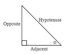
2nd: The Opposite and Adjacent sides are then defined by the angle you are going to work with. One of the sides will be opposite this angle and the other side will be beside (adjacent to) this side.
For example: The following sides are defined by the right angle and the angle you are going to work with Ø. You will have to define the adjacent and opposite sides for every right triangle you work with.
The other right angled trigonometric ratios are the reciprocals of Sine, Cosine and Tangent:
Cosecant = 1/Sine Secant = 1/Cosine Cotangent = 1/Tangent
or formally defined as:
[latex]Cosecant =\dfrac{Hypotenuse}{Opposite}[/latex] [latex]Secant =\dfrac{Hypotenuse}{Adjacent}[/latex] [latex]Cotangent =\dfrac{Adjacent}{Opposite}[/latex]
You often see these equations shortened to:
[latex]Csc =\dfrac{Hyp}{Opp}[/latex] [latex]Sec =\dfrac{Cot}{Adj}[/latex] [latex]Cot =\dfrac{Adj}{Opp}[/latex]
These reciprocal trigonometric functions are commonly used in calculus, specifically in integration and when working with polar coordinates. Anyone taking higher levels of mathematics will encounter these reciprocal trigonometric functions.
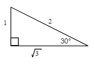
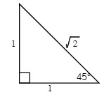
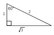
Using the Pythagorean Theorem for 30°, 45° and 60° right angle triangles, you can get the exact values of the trigonometric relationship (and the reciprocal values). Standard exams require students to draw these 30°, 45° and 60° right angle triangles and use the side lengths to generate exact values.
Trigonometric tables are commonly used as approximations of the trig ratios of standard angles from 1° to 90°. For these tables you choose the value that lines up the trigonometric function you wish to use with the angle that you are using. Basic scientific calculators have essentially made these tables obsolete.
EXAMPLE 7.1.1
Find the values that correspond to the following trigonometric functions and angles:
Sin 19° = x Cos 67° = y Tan 38° = z
Solution:
x = 0.326y = 0.391z = 0.781
It is also possible to work in reverse, i.e., given the trigonometric ratio of two sides, you can find the angle that you are working with.
EXAMPLE 7.1.2
Find the angles that correspond to the following trigonometric values:
Sin Ø = 0.829 Cos Ø = 0.940 Tan Ø = 3.732
Solution:
Ø = 56° Ø = 20° Ø = 75°
Sometimes you do not have a value that matches up. For these cases you choose the value that is closest to what you have.
EXAMPLE 7.1.3
Find the angles that are closest to the following trigonometric values:
Sin Ø = 0.297 Cos Ø = 0.380 Tan Ø = 0.635
Solution:
Ø = 17° Ø = 68° Ø = 32°
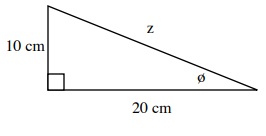
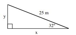
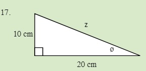
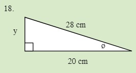
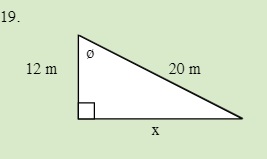
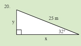
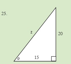
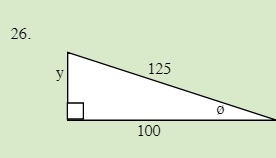
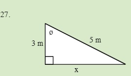
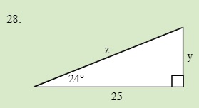
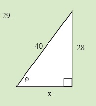
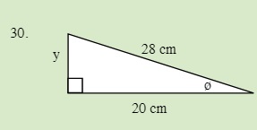
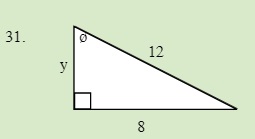
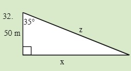
EXAMPLE 7.1.4
EXAMPLE 7.1.5
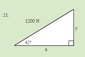
Solve for the unknown sides in the following triangle.
Trigonometric Tables
| Angle | Sin | Cos | Tan | Cse | Angle | Sin | Cos | Tan | Cse |
|---|---|---|---|---|---|---|---|---|---|
| 1 | 0.017 | 1.000 | 0.17 | 57.299 | 46 | 0.719 | 0.695 | 1.036 | 1.390 |
| 2 | 0.035 | 0.999 | 0.035 | 28.654 | 47 | 0.731 | 0.682 | 1.072 | 1.36 |
| 3 | 0.052 | 0.999 | 0.052 | 19.107 | 48 | 0.743 | 0.669 | 1.111 | 1.346 |
| 4 | 0.070 | 0.998 | 0.070 | 14.336 | 49 | 0.755 | 0.656 | 1.150 | 1.325 |
| 5 | 0.087 | 0.996 | 0.087 | 11.474 | 50 | 0.766 | 0.643 | 1.192 | 1.305 |
| 6 | 0.105 | 0.995 | 0.105 | 9.567 | 51 | 0.777 | 0.629 | 1.235 | 1.287 |
| 7 | 0.122 | 0.993 | 0.123 | 8.206 | 52 | 0.788 | 0.616 | 1.280 | 1.269 |
| 8 | 0.139 | 0.990 | 0.141 | 7.185 | 53 | 0.799 | 0.602 | 1.327 | 1.252 |
| 9 | 0.156 | 0.988 | 0.158 | 6.392 | 54 | 0.809 | 0.588 | 1.376 | 1.236 |
| 10 | 0.174 | 0.985 | 0.176 | 5.759 | 55 | 0.819 | 0.574 | 1.428 | 1.221 |
| 11 | 0.191 | 0.982 | 0.194 | 5.241 | 56 | 0.829 | 0.559 | 1.483 | 1.206 |
| 12 | 0.208 | 0.978 | 0.213 | 4.810 | 57 | 0.839 | 0.545 | 1.540 | 1.192 |
| 13 | 0.225 | 0.974 | 0.231 | 4.445 | 58 | 0.848 | 0.530 | 1.600 | 1.179 |
| 14 | 0.242 | 0.970 | 0.249 | 4.134 | 59 | 0.848 | 0.530 | 1.600 | 1.179 |
| 15 | 0.259 | 0.966 | 0.268 | 3.864 | 60 | 0.866 | 0.500 | 1.732 | 1.155 |
| 16 | 0.276 | 0.961 | 0.287 | 3.628 | 61 | 0.875 | 0.485 | 1.804 | 1.143 |
| 17 | 0.292 | 0.956 | 0.306 | 3.420 | 62 | 0.883 | 0.469 | 1.881 | 1.133 |
| 18 | 0.309 | 0.951 | 0.325 | 3.236 | 63 | 0.891 | 0.454 | 1.963 | 1.122 |
| 19 | 0.326 | 0.946 | 0.344 | 3.072 | 64 | 0.899 | 0.438 | 2.050 | 1.113 |
| 20 | 0.342 | 0.940 | 0.364 | 2.924 | 65 | 0.906 | 0.423 | 2.145 | 1.103 |
| 21 | 0.358 | 0.934 | 0.384 | 2.790 | 66 | 0.914 | 0.407 | 2.246 | 1.095 |
| 22 | 0.375 | 0.927 | 0.404 | 2.669 | 67 | 0.921 | 0.391 | 2.356 | 1.086 |
| 23 | 0.391 | 0.921 | 0.424 | 2.559 | 68 | 0.927 | 0.375 | 2.475 | 1.079 |
| 24 | 0.407 | 0.914 | 0.445 | 2.459 | 69 | 0.934 | 0.358 | 2.605 | 1.071 |
| 25 | 0.423 | 0.906 | 0.466 | 2.366 | 70 | 0.940 | 0.342 | 2.747 | 1.064 |
| 26 | 0.438 | 0.899 | 0.488 | 2.281 | 71 | 0.946 | 0.326 | 2.904 | 1.058 |
| 27 | 0.454 | 0.891 | 0.510 | 2.203 | 72 | 0.951 | 0.309 | 3.078 | 1.051 |
| 28 | 0.469 | 0.883 | 0.532 | 2.130 | 73 | 0.956 | 0.292 | 3.271 | 1.046 |
| 29 | 0.485 | 0.875 | 0.554 | 2.063 | 74 | 0.961 | 0.276 | 3.487 | 1.040 |
| 30 | 0.500 | 0.866 | 0.577 | 2.000 | 75 | 0.966 | 0.259 | 3.732 | 1.035 |
| 31 | 0.515 | 0.857 | 0.601 | 1.942 | 76 | 0.970 | 0.242 | 4.011 | 1.031 |
| 32 | 0.530 | 0.848 | 0.625 | 1.887 | 77 | 0.974 | 0.225 | 4.331 | 1.026 |
| 33 | 0.545 | 0.839 | 0.649 | 1.836 | 78 | 0.978 | 0.208 | 4.705 | 1.022 |
| 34 | 0.559 | 0.829 | 0.675 | 1.788 | 79 | 0.982 | 0.191 | 5.145 | 1.019 |
| 35 | 0.574 | 0.819 | 0.700 | 1.743 | 80 | 0.985 | 0.174 | 5.671 | 1.015 |
| 36 | 0.588 | 0.809 | 0.727 | 1.701 | 81 | 0.988 | 0.156 | 6.314 | 1.012 |
| 37 | 0.602 | 0.799 | 0.754 | 1.662 | 82 | 0.990 | 0.139 | 7.115 | 1.010 |
| 38 | 0.616 | 0.788 | 0.781 | 1.624 | 83 | 0.993 | 0.122 | 8.144 | 1.088 |
| 39 | 0.629 | 0.777 | 0.810 | 1.589 | 84 | 0.995 | 0.105 | 9.514 | 1.006 |
| 40 | 0.643 | 0.766 | 0.839 | 1.556 | 85 | 0.996 | 0.087 | 11.430 | 1.004 |
| 41 | 0.656 | 0.755 | 0.869 | .1524 | 86 | 0.998 | 0.070 | 14.301 | 1.002 |
| 42 | 0.669 | 0.743 | 0.900 | 1.494 | 87 | 0.999 | 0.052 | 19.081 | 1.001 |
| 43 | 0.682 | 0.731 | 0.933 | 1.466 | 88 | 0.999 | 0.035 | 28.636 | 1.001 |
| 44 | 0.695 | 0.719 | 0.;966 | 1.440 | 89 | 1.000 | 0.017 | 57.290 | 1.000 |
| 45 | 0.707 | 0.707 | 1.000 | 1.414 | 90 | 1.000 | 0.000 | 1.000 |
QUESTIONS 7.1 Right Angle Trigonometric Functions
7.2 Vector Resolution into Components 6
Through practice you will be able to quickly resolve angled vectors using right triangle trigonometry. For example given a force vector of 100 N angled at 42° from the horizontal, you can break it up into vertical and horizontal components using the Sine and Cosine functions. In this instance the vector components are as follows:
Quick Resolution: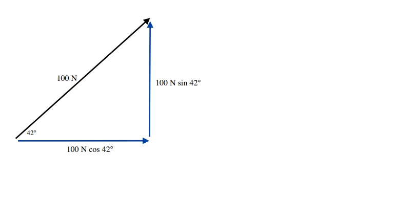
F = 100 N
Fx = 100 N cos 42° (≈ 74 N)
Fy = 100 N sin 42° (≈ 70 N)
A more detailed resolution is:
Fx Cos 42° = Fx . which when isolated leaves us with Fx = 100 N cos 42°
100 N
Fy Sin 42° = Fx . which when isolated leaves us with Fy = 100 N sin 42°
100 N
The easy way to remember this is when the vector magnitude is known then the opposite side vector is the sine of the vector angle and the adjacent side vector is the cosine of the vector angle.
To illustrate the opposite, when both vector components are known, the angle of the resultant vector can be found using the tangent function and the magnitude of the vector by using the Pythagorean Theorem. For this, one generally uses a more traditional approach. Consider the following example:
The magnitude of the net force is 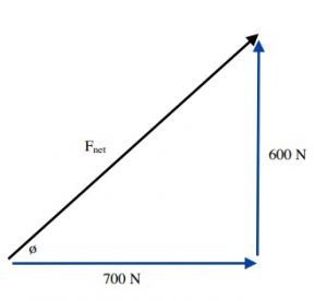
(Fnet)2 = (600 N)2 + (700 N)2
(Fnet)2 = 360 000 N2 + 490 000 N2
(Fnet)2 = 850 000 N2
Fnet = 922 N ( ≈ 920 N)
The angle this makes is
Tan ø =[latex]\dfrac{\text{600 N}}{\text{700 N}}[/latex]
Tan ø = 0.8571
ø = Tan-1 0.8571
ø = 40.6° (≈ 41°)
The main purpose of this section is for you to be able to quickly resolve a vector with angle into components.
EXAMPLE 7.2.1
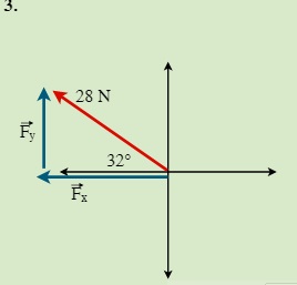
Resolve the following vectors and angles into components.
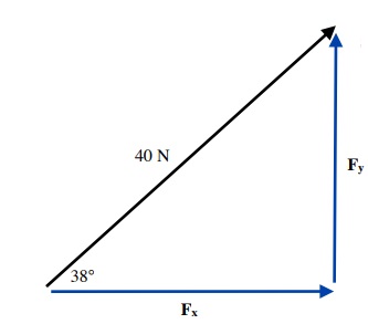
Solution
Fx = 40 N cos 38° or 31.5° (≈ 32 N)
Fy = 40 N sin 38° or 24.6° (≈ 25 N)
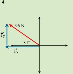
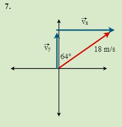
EXAMPLE 7.2.2
Resolve the following vectors and angles into components.
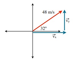
[latex]\overrightarrow{v}_y=\text{ 48 m/s sin 32° or 25.4 m/s } (\approx25 m/s)[/latex]
[latex]\overrightarrow{v}_x =\text{ 48 m/s cos 32° or 40.7 m/s } (\approx41 m/s)[/latex]
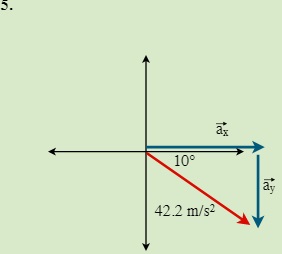
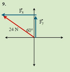
EXAMPLE 7.2.3
Resolve the following vectors and angles into components.
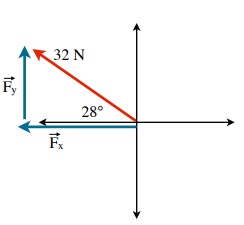
[latex]\overrightarrow{F}_{y} =\text{32 m/s sin 28° or 15 m/s}[/latex]
[latex]\overrightarrow{F}_{x} =\text{32 m/s cos 28° or 15 m/s}[/latex]
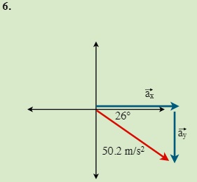
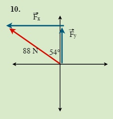
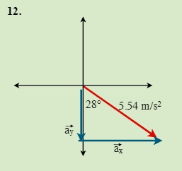
EXAMPLE 7.2.4
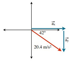
[latex]\overrightarrow{a}_{y} =\text{20.4 m/s}^{2}\text{ sin 42° or (-)14 m/s}^{2}[/latex]
[latex]\overrightarrow{a}_{x} =\text{20.4 m/s}^{2}\text{ cos 42° or 15 m/s}^{2}[/latex]
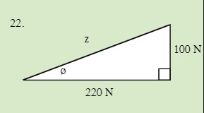
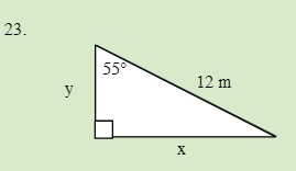
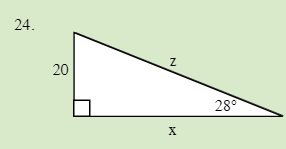
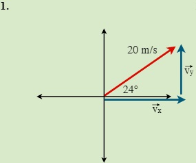
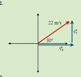
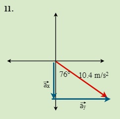
QUESTIONS 7.2 Break the following vectors into components (not drawn to scale)

7.3 Static Equilibrium (Concurrent Forces) 7
Static equilibrium is one of the requirements of architecture. Engineering tools and techniques have been employed since ancient times to create buildings that are statically safe from collapse. In short, structural design must work to counteract the effects of gravity, storms and earthquakes to name a few of the forces that can act on a structure.


The bridge above was thought to have been built during the reign of Augustus (27 BC- 14AD) as an aqueduct to supply water to the town of Tarraco in Catalonia, Spain. This structure is 249 m in length, and comprised of a series of free-standing stone arches that have the same radius of 5.9 ± 0.15 m. Of the 931 surviving Roman bridge structures, the largest of these is the Puente Romano bridge in Merida, Spain with a length of 792 m.
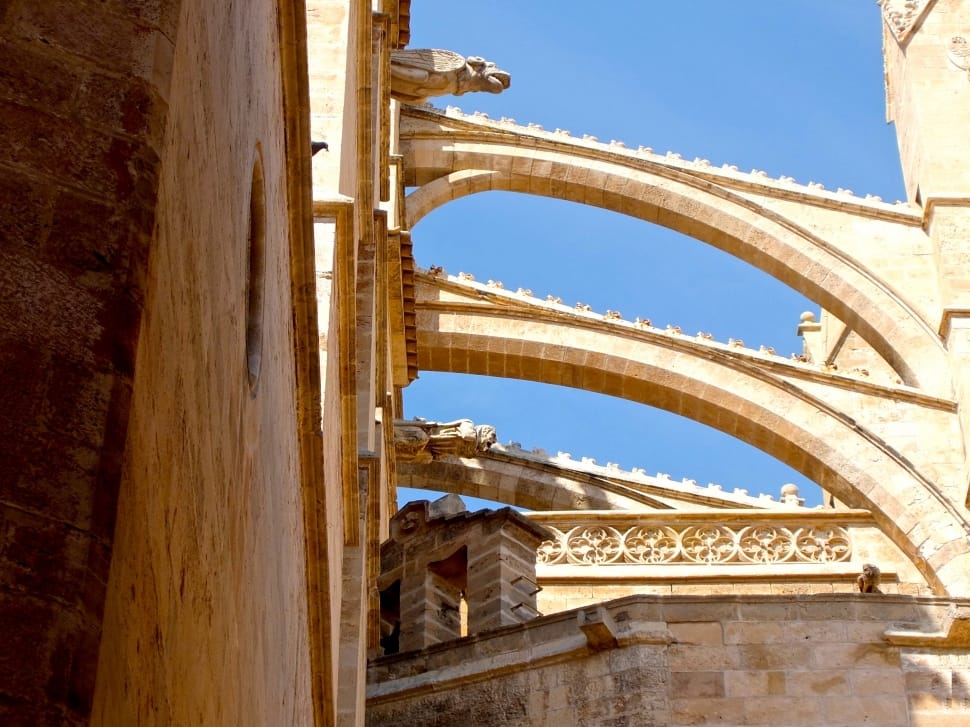
The arch design used in Roman bridges is one that is found in nature, such as the Azure Window shown to the right and located in Malta. The success of the strength in the design of arch structures is how the force from the weight of the bridge is carried outward along the curve of the arch and is balanced by the supports anchoring either end.
The flying buttress design used in Notre Dame Cathedral consists of half arches placed on either side of the building to support the weight and wind shears acting on the central dome covering the building. This technique of balancing forces opened up the walls of the building to construct windows to be constructed in the walls and let in light while supporting the weight of the roof.
- The picture above I did not find at the Design Technology website. We can contact them at ajdavies1967@hotmail.com
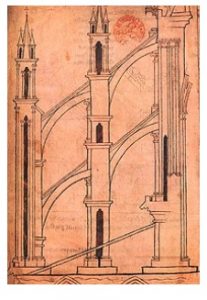
The sketch shown above is by Villard de Honnecourt (1225-1235). It is part of a collection of works showing various designs of devices he saw while traveling though Medieval Europe.
The forces that act in an arch bridge are illustrated in the images8 shown below showing the force vectors acting in the Action Force (Load) and the Reaction Force (Support for the Load).
Conceptual Origins
The term equilibrium9 originates from the Latin acqui and libra, meaning equal balance. When used in physics concepts, objects in a state of equilibrium refer to a balancing of forces acting on the object. The basic concept that grounds equilibrium is that all forces acting on a point in an object sum to zero. This is the embodiment of Newton’s First Law.
To recap: Newton’s First Law states that every object will remain at rest or in uniform motion in a straight line unless compelled to change its state by the action of an external force. This is normally taken as the definition of inertia. If there is no net force acting on an object (if all the external forces cancel each other out) then the object will maintain a constant velocity. If that velocity is zero, then the object remains at rest. If an external force is applied, the velocity will change because of the force.
From the Latin version of Newton’s Principia, his first law reads as:
Lex I: Corpus omne perseverare in statu uo quiescendi vel movendi uniformiter in directum, nisi quatenus a viribus impressis cogitur statum illum mutare.
Translated to English, this reads:
Law I: Every body persists in its state of being at rest or of moving uniformly straight forward, except insofar as it is compelled to change its state by force impressed.
Newton then goes on to expand on his First Law with:
Projectiles persevere in their motions, so far as they are not retarded by the resistance of the air, or impelled downwards by the force of gravity. A top, whose parts by their cohesion are perpetually drawn aside from rectilinear motion, does not cease its rotation, otherwise than as it is retarded by the air. The greater bodies of the planets and comets, meeting with less resistance in more free spaces, preserve their motions both progressive and circular for a much longer time.
One of the challenges to the interpretation of Newton’s Laws is that he appears to have written these Laws following the style of earlier Greek philosophers, such as Euclid. Historians have suggested that Newton’s First Law is simply a natural deduction of his Second Law, since Newton’s writings include no frames of reference.
Equilibrium is explored in three different ways in this chapter: Translational, Static and Rotational, all relating to the balancing of forces that act on an object or a structure. Equilibrium is a very important concept, and you should encounter a number of different ways that explore equilibrium in specialized fields.
Translational Equilibrium occurs when no net or resultant force is acting on an object. The means that the sum of all forces that are acting will equal 0 N. Newton’s First Law interprets this to mean that if the object is at rest, it will remain at rest and if the object is in motion, it will remain in that exact state of motion.
Rotational Equilibrium requires that the object is non-rotating. This necessitates that all forces causing it to rotate (torques) will sum to zero. Newton’s First Law interprets this to mean that if the object is at rest, not-rotating, it will remain at rest and not-rotating. If the object is rotating, it will remain in that exact state of rotation, neither speeding up nor slowing down.
Static Equilibrium is a special case of Translational and Rotational Equilibrium and occurs when the net force or resultant force acting on an object sums to zero and the object is neither moving in any direction nor rotating. Static Equilibrium requires that the object in question is at rest and remains at rest.

- To use the picture above we will have to fill in a request at this link https://shmoop.zendesk.com/hc/en-us/requests/new
When we look at the effect of forces acting on a body, there are five commonly observed actions10. You will be encountering the first two of these (compression (C) and Tension (T) while working on the problems in this chapter.
Free Body Diagrams 11
One of the standard tools used to analyze forces in equilibrium is the Free Body Diagram.12 Free body diagrams show the magnitude and direction of all forces that act on a body in a given situation. In many cases these diagrams are drawn to scale with the length of the arrow in scale to the magnitude of the force and the angle of this force accurately positioned. Learning to draw a free body diagram is important for one to be able to work through questions in statics, dynamics and a few other fields of classical mechanics.
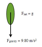
Using the free body diagram as a tool, one is able to easily visualize whether or not the forces acting on an object add to zero (Fnet = 0), meaning that the object is in static equilibrium and not moving. If the forces acting on the body do not add to zero (Fnet ≠ 0) it will accelerate.
Hyperphysics lists a number of common forces that you can encounter where free body diagrams assist in working out the intricacies of the problem. In Chapter 6, you encountered weight (w, Fg), which is a force vector directed straight down towards the Earth’s center. In this chapter you will use another force vector called Tension (T, Ft). Tension is the force that exists in strings, cables, ropes or beams that are acting to apply a force on an external object. Tension in these examples includes the forces transmitted by the cable, rope, string or beam, and acts in the direction these are pulling or pushing. In the examples that follow, this tension balances the weight (simplest) which becomes more complicated when multiple tensions act on an external object.
Other common forces that you will encounter:
The Normal Force (N, Fn) which can be explained as the force exerted by a surface tangentially away from the surface to support an object.
Frictional Force (f, Ff) which is the force acting between two surfaces and is generally opposite to the direction the object is moving or accelerating (but this is not always true).
Elastic Forces (Fe, Fs) are the forces exerted by springs or rubber bands, etc., when they are stretched (or compressed in some cases). The force in these instances acts in the direction of the stretch or compression.
Buoyancy (B, Fb) are the forces that act on objects that are immersed or suspended in a fluid. The direction of buoyancy is always upwards and away from the center of the Earth.
Drag or Air Resistance (R, D, Fd, Fair)is the force that acts on any object that is moving through a fluid, be it liquid or gaseous. This force will generally be acting opposite to the direction that the object is moving (opposite to the velocity).
Lift (L, Fl) is the force that acts on an object that is tangential to its movement through a fluid, meaning that as the object is moving forward through a fluid, the lift will act at 90° to the direction of the object’s velocity.
Thrust (T, Ft) is the action-reaction force that results from pushing a fluid in one direction (generally backwards) that allows the object doing this pushing to move in the opposite direction.
In all cases, combinations of the above forces can be acting on some object requiring one to find the net result of forces (Fnet) acting on the object. All these forces are in Newtons (N).
The following examples will illustrate how one can draw a free body diagram of the forces acting on a body.
EXAMPLE 7.3.1
Consider a parachutist:
(i) First starts to fall (ii) Reaches terminal velocity
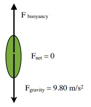
EXAMPLE 7.3.2
A person floating in a lake
The principle used to draw these diagrams is the same when you encounter more than two forces acting on an object. Two cables supporting an object at rest or moving at a constant velocity (Fnet = 0) would show up as two forces acting in unison to balance the weight or force of gravity pulling down on the object. If these cables are acting to accelerate the object either up, down or to one side (Fnet ≠ 0) then the forces acting on the object would show some imbalance. In all cases, the force arrows will act in the directions that the forces act on the object.
EXAMPLE 7.3.3
Suppose you have a box suspended in air by two cables, as shown below.
If we were to redraw this using Force vectors, it would look like
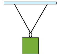
To properly analyze this diagram we would need both the magnitudes and directions of all forces acting on the box. (Forces are generally termed Tensions when these forces are pulling on the cable. This is compared to a beam that can be experiencing a force acting to compress it.)
This diagram to the right can be further reduced to
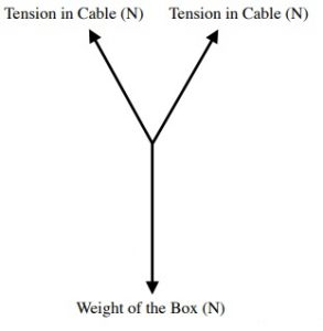

Trigonometry would be used at this point to break the two cable tensions (T1 & T2) into vector components. The rest of the solution would use algebra to balance the forces acting on the box.
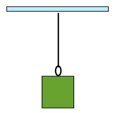
EXAMPLE 7.3.4
Find the tension in a cable supporting a single box of 25 kg in Static Equilibrium.
The sketch and the free body diagrams for this example are:
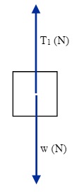
The solution for this requires that the forces acting on the box must sum to zero. In an equation this looks like:
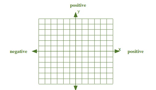
To solve this problem, assign cartesian directions as you would on a graph. For y-direction, up is positive and down is negative and for the x-direction, right is positive and left is negative.
Using this vector notation, the solution is:
[latex]\Sigma\overrightarrow{F}_y =\text{0 N}[/latex]
T1 + w = 0 N
T1 + (25 kg)(- 9.8 m/s2) = 0 N
T1 – 245 N = 0 N
T1 = 245 N (≈ 250 N) The direction of this force is upwards.
EXAMPLE 7.3.5
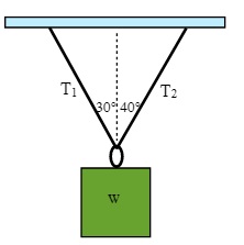
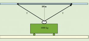
Find the tension in the two cables supporting a single crate of 100 kg in Static Equilibrium as shown in the diagram below to the right.
The Free Body diagram of this problem looks like
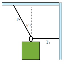
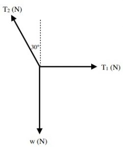
These forces are acting in two directions: ± x and ± y. The solution for this requires balancing these forces in two directions.
[latex]\Sigma\overrightarrow{F}_{x} =\text{ 0 N and }\Sigma\overrightarrow{F}_{y} = 0[/latex]
Weight = (100 kg)(- 9.8 m/s2) or – 980 N in the y-direction
Since cable 2 is the only cable supporting the crate, we know that the tension in the cable in the y-direction must be + 980 N. The sketch of this looks like this:
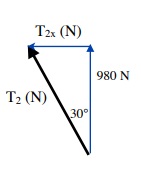
Trigonometry is now used to find the tension of cable 2 in the x direction (T2x)
Tan 30° = T2x
980 N
T2x = 980 N Tan 30°
T2x = – 566 N (≈ – 570 N) negative x-direction
Now, the total Tension of cable 2 is and, the Tension of cable 1 is
[latex]\text{Cos 30°} =\dfrac{\text{980 N}}{T_2}[/latex] T1 = 566 N (≈570 N)
(equal and opposite to T2x)
[latex]T_{2} =\dfrac{\text{980 N}}{\text{Cos 30°}}[/latex]
T2 = 1132 N (≈ 1100 N)
Putting all of this in a free body diagram yields
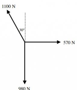
When summing up the forces:
[latex]\Sigma\overrightarrow{F}_{x} =\text{ 0 N and }\Sigma\overrightarrow{F}_{y} =\text{ 0 C}[/latex]
[latex]\Sigma\overrightarrow{F}_{y} =\text{ 0 N}[/latex]
T2y + w = 0 N
980 N – 980 N = 0 N
[latex]\Sigma\overrightarrow{F}_{x} =\text{ 0 N}[/latex]
T2x + T1 = 0 N
– 566 N + 566 N = 0 N∑ Fx = 0 N and ∑ Fy = 0 C
EXAMPLE 7.3.6
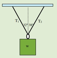
Find the tension in the two cables supporting a single box of 420 kg in Static Equilibrium as shown in the diagram below and to the right.
The free body diagram for this problem looks like:
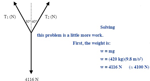
Solving this problem is a little more work.
First, the weight is:
w = mg
w = (420 kg)(9.8 m/s2)
w = 4116 N (≈ 4100 N)
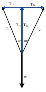
Summing up the Forces acting on the box:
In the y direction: T1y + T2y + w = 0 N
In the x direction: T1x + T2x = 0 N
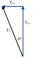
Finding what we know about the Tensions
Sin 30° = T1x ÷ T1
or … T1x = T1 Sin 30°
T1x = 0.500 T2
Cos 30° = T1y ÷ T1
or … T1y = T1 Cos 30°
T1y = 0.866 T1
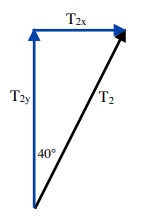
Sin 40° = T2x ÷ T2
or … T2x = T2 Sin 40°
T2x = 0.643 T2
Cos 40° = T2y ÷ T2
or … T2y = T2 Cos 40°
T12y = 0.766 T2
Balancing all Forces
x direction:0 N = T1x + T2x 0 N = 0.500 T1 – 0.643 T2
y direction: 0 N = T1y + T2y + w or 0.866 T1 + 0.766 T2 = 4116 N
Now, use substitution to solve this system of two equations
First: Isolate T1 0 N = 0.643 T1 – 0.500 T2 or
0.500 T1 = 0.643 T2
T1 = 0.643 T2 or 1.29 T2
0.500
Second: Substitute for T2 0.866 T1 + 0.766 T2 = 4116 N
0.866 (1.29 T2) + 0.766 T2 = 4116 N
1.12 T2 + 0.766 T2 = 4116 N
1.886 T2 = 4116 N
T2 = 4116 N ÷ 1.462 or 2182 N (≈ 2200 N)
Finally: T1 = 1.29 T2 or T1 = (1.29)(2182 N)
T1 = 2815 N (≈ 2800 N)
EXAMPLE 7.3.7
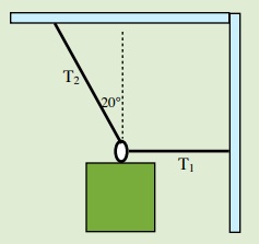
Find the tension in the cable and the reactive force from the beam supporting a single crate of 500 kg in Static Equilibrium as shown in the diagram below to the right.
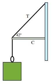
Weight = (500 kg)(- 9.8 m/s2) or – 4900 N
Conditions for equilibrium
[latex]\Sigma\overrightarrow{F}_{x} =\text{ 0 N}[/latex] and [latex]\Sigma\overrightarrow{F}_{y} = 0[/latex]
Since this cable is the only force supporting the crate, we know that the tension in the cable in the y-direction must be + 4900 N
Ty = + 4900 N
Trigonometry is now used to find the tension of the cable in the x direction (Tx)
[latex]\text{Tan 42°} =\dfrac{\text{4900 N}}{T_{x}}[/latex]
[latex]T_{x} =\dfrac{\text{4900 N}}{\text{Tan 42°}}[/latex]
Tx = 5442 N (≈ 5400 N) … positive x-direction
Now, the total Tension of the cable is
[latex]\text{Sin 42° =}\dfrac{\text{4900 N}}{T}[/latex]
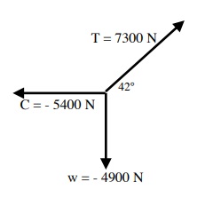
[latex]T =\dfrac{\text{4900 N}}{\text{Sin 42°}}[/latex]
T = 7323 N ( ≈ 7300 N)
The reactive force from the beam is
C = – 5442 N (≈ – 5400 N)
(equal and opposite to Tx)
QUESTIONS 7.3 Find the forces required for static equilibrium in the following problems.
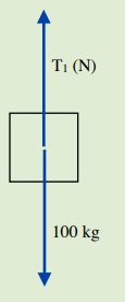
1. Find the tension in a cable supporting a single box of 100 kg in static equilibrium.
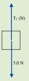
2. Find the tension in a cable supporting a single box weighing 5.0 N in static equilibrium.
3. Find the tension in the two cables supporting a single crate of mass 50 kg in static
equilibrium as shown in the diagram below to the right.
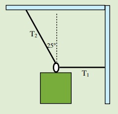
4. Find the tension in the two cables supporting a single crate of 250 kg in static equilibrium as shown in the diagram below to the right.
5. Find the tension in the two cables supporting a single crate of 120 kg in static equilibrium as shown in the diagram below and to the right.
6. Find the tension in the two cables supporting a single crate of 1200 kg in static equilibrium as shown in the diagram below and to the right.
7. Find the tension in the cable and the reactive force from the beam supporting a single crate of 420 kg in static equilibrium as shown in the diagram below to the right.
8. If the maximum recommended tension in the cable is 12 000 N, find the reactive force
from the beam that would be needed to support this maximum in static equilibrium as shown in the diagram below to the right.
QUESTIONS 7.4.1 A cable that has a maximum load tension of 50 000 N is slowly lifting a
heavy crate straight upwards. (i) How close to the top can the crate be safely lifted?
(ii) What is the mass that can be lifted to within 10 cm from the top?
REFERENCES:
